
The Experiment
Experimental constraints
In order to test the full capabilities of the TerrusM, the experiment was conducted in a challenging area with a significant distance between buildings and the forest. SLAM systems tend to perform better with more detail. As a further restraint, the TerrusM was chosen over the TerrusS in order to solely test the system’s odometry without the aid of GPS.
The operator started each scan 400m away from the end of the street and traversed down the right side of the road, simulating the movement of a car. The operator then turned around at the end of the roundabout and travelled back on the left side of the road.
While a static scanner may have required several set-ups and hours to scan this location, the six scans for this experiment were completed in just one and a half hours (15 minutes per scan). Noting that these results were captured using a backpack application and may be captured faster by attaching the system to a car. Further demonstrating the efficiency and convenience of using a mobile system.
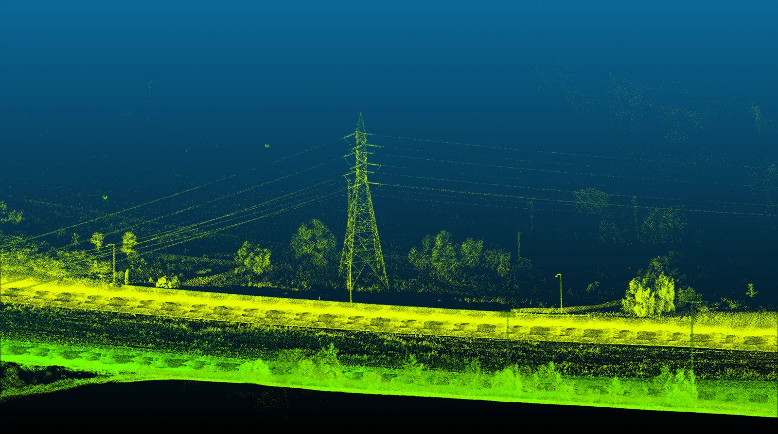
Capturing Wolston Rd
To begin this experiment the AutoMap team travelled to a local cul-de-sac in Sumner Park, Queensland. Throughout the day, the operators traversed the 400m dead end six times in a row with the TerrusM. Of traversal was captured in a single direction only.
After completing the scans, the resulting maps were imported and aligned into a point cloud software and underwent a cloud-to-cloud comparison process. This enabled the program to quantify the error between each set of pointclouds.
The results of the comparison are presented in the images on the right. The images illustrate the results of two compared unique pointclouds shaded from green (low error) to red (high error).
Comparative Analysis
To analyze the error between the different sets of maps, cloud-to-cloud error plot graphs (left) were generated. These graphs allow for the breakdown of the error in distance between each point in the pointclouds, measured in millimetres.
These results of all three comparisons clearly present that across all six maps, there was minimal error between scans. 25% of the captured points had a differential error of less than 0.007m (7mm), and 50% had a difference of less than 2.5cm across the three map sessions. The error plot graphs on the left display the distribution of differential error for each of the six scan sessions.
During the experiment, it was observed that data with higher accuracy (represented by “GREEN” in the error plot) typically corresponded to data captured of static features that were closer to the laser. In contrast, trees and other moving features had a larger amount of differential error, as seen in the “RED” colouration of the error plots and maps. The maximum difference across all scans was limited to a few points with a 0.20m difference. This is likely due to the presence of moving objects in the area, such as trees and road traffic.